Fitting an image

The image task fits an INR \([-1, 1]^2 \to \mathbb{R}^3\) to one image and scores it on every pixel. This tutorial follows configs/image.yaml and scripts/train_image.py, so what you run here is what the benchmark ran.

kodim19 at about 197k parameters: two regions magnified for every featured model, above each model's |error|, with its PSNR over the whole image.

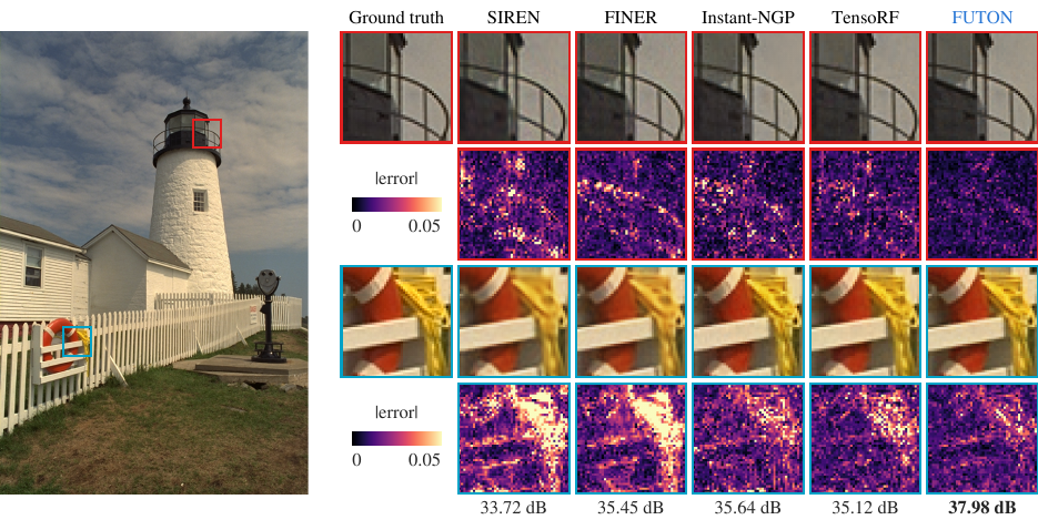
Data

import torch
import inro

path = "data/Kodak/kodim19.png"
train_set = inro.ImageCoordinateDataset(path)  # the whole image at every step
eval_set = inro.ImageCoordinateDataset(path)
H, W = eval_set.grid_size

Each access is one training step, and the benchmark trains on the whole image at every step, as the papers of the SIREN family do. Other options:

Option	Effect
subsample	Draws a fresh random share of the pixels instead
max_samples	Caps the draw, for images too large for one step
mode="L"	Loads a grayscale image (out_features=1)
item_id	Names the signal in logs when you pass a tensor or PIL image instead of a path

Models at equal size

Each benchmark model holds about 197k parameters. FUTON's basis size follows the image, half the sampling resolution per axis, and its grid_size declares the pixel grid, on which the basis is evaluated once and each point reads its row. The first layer of its MLP head reads a batch that covers the image off the grid in one contraction.

FUTONSIRENFINERInstant-NGPTensoRF

futon = inro.FUTON(
    2, 3,
    basis=("cosine", {"num_components": [H // 2, W // 2], "grid_size": (H, W)}),
    combiner=("cp", {"rank": 280}),
    head=("mlp", {"hidden_layers": 1, "hidden_features": 64}),
    output_activation=torch.tanh,
)

siren = inro.SIREN(2, 3, hidden_features=256, hidden_layers=4, omega=30.0,
                   output_activation=torch.tanh)

finer = inro.FINER(2, 3, hidden_features=256, hidden_layers=4, omega=30.0,
                   output_activation=torch.tanh)

ngp = inro.InstantNGP(
    2, 3,
    num_levels=20, features_per_level=2, log2_hashmap_size=13,
    base_resolution=16, max_resolution=max(H, W) // 2,
    hidden_features=64, hidden_layers=2, output_activation=torch.tanh,
)

tensorf = inro.TensoRF(2, 3, rank=176, resolution=256, mode="cp",
                       hidden_features=256, hidden_layers=2,
                       output_activation=torch.tanh)

The learning rate matters. Every model trains with PyTorch's default Adam, at these rates:

Model	FUTON	SIREN	FINER	Instant-NGP	TensoRF
Learning rate	1e-1	1e-3	1e-3	3e-2	3e-2

configs/image.yaml lists all thirteen models with their rates and, where a setting departs from the authors' code, a comment saying why. Use inro.count_parameters(model, trainable_only=False) when you change a size.

Training

result = inro.train(
    futon,
    train_set,
    eval_set,
    num_steps=1000,
    lr=1e-1,
    metrics={"psnr": inro.psnr, "ssim": inro.ssim, "ms_ssim": inro.ms_ssim, "lpips": inro.lpips},
    log_interval=50,
    eval_interval=50,
    log_dir="logs/tutorial/kodim19/FUTON",
)

The metrics run on the uint8 reconstruction against the original every 50 steps.

Tip

LPIPS is the slow one, since it runs a VGG network each time. Leave it out of metrics while iterating, and compute it once at the end with inro.evaluate.

Learning curves

history is a list of records, one per logged step, with the evaluation metrics under "eval":

import pandas as pd

curve = pd.DataFrame(
    {"step": h["step"], "time": h["elapsed"], **h["eval"]}
    for h in result["history"] if "eval" in h
)
curve.plot(x="time", y="psnr")

The same curve over the 24 Kodak images, for FUTON and the strongest model of each family.

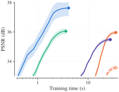
inro.LinePlot wraps seaborn for the multi-model case: collect one record per model and step and call LinePlot(records).plot(x="time", y="psnr", hue="model"). The notebook notebooks/image_representation.ipynb collects such records for seven models and draws them with seaborn itself.

Reconstruction

output = inro.chunked_inference(futon, eval_set.input, chunk_size=65536)  # (H, W, 3)
image = eval_set.postprocess(output.cpu())                                # uint8 (3, H, W)
eval_set.save(image, "kodim19_futon.png")

inro.evaluate(model, eval_set, metrics=..., ckpt_path="logs/.../checkpoint.pt", log_dir=...) does the same from a checkpoint and writes the reconstruction beside the logs.

The benchmark script

scripts/train_image.py runs every model of the config on every image under data/Kodak/, writes each run to logs/image/<image>/<model>/, and skips runs that already have a results.json:

python scripts/train_image.py                                        # all images, all models
python scripts/train_image.py --data data/Kodak/kodim19.png --models FUTON SIREN
python scripts/train_image.py --set train.num_steps=500 --log-dir logs/short

Sizes in the config may be expressions in the image height H and width W, such as max(H, W) // 2. See Reproducing the paper for the full command-line interface.